Quantifying product impact

A guide to measure and standardize experiment results for product teams

Defining product impact

Most of the best product teams in software have some way to show how their work is affecting change. There are many avenues to do this, but I wanted to go through my team’s methodology as I have found it invaluable for achieving operational success. We defined product impact as:

Metric change x Affected population = Impact

Although this formula seems simple let’s talk through the different pieces. When code is shipped into production typically there is some effect that occurs for a number of end users. Our goal is to understand what this effect is and have a shared language on how to describe it. We call this effect “impact”. If a code change or product is particularly “impactful” it has made a large change to the collective user experience.

“Metric change” represents the change in the user’s experience by one metric, and it is often used alone to determine product impact. For example: a common procedure might be to look at a metric like “add-to-cart actions”. If there are more add-to-cart actions in enabled compared to control, then enabled should be shipped to all users. However, this procedure stops short and leaves out an important piece of information for us to understand impact. In order to compare this product change to other product changes, we have to know not only how much the users were impacted, but how many users were impacted by the change. Knowing those two pieces of information together allows us to understand which changes have a high ROI (where the “Return” is user experience and the “I” is engineering time)

The affected population is simply how many users will be exposed to this feature over a set amount of time. If a change was made on the settings page of an app, the affected population would be every user who landed on the settings page over X days.

Let’s go through an example of how the formula is used:

The acquisition team of a series B startup wants to create a new way to add products to a user’s cart. The team comes up with an awesome idea and decides to launch it behind an experiment.

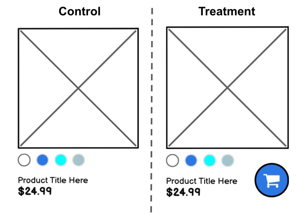
They see a 10% absolute increase in the number of users performing an add to cart (ATC) action with a total affected population of 100K users over 90 days. They use the product impact formula and see a result of 10K more users performing an ATC action over the next 90 days. They expect ~111 additional users to ATC per day as a result of this experiment.

With this measurement of impact the acquisition team can easily compare their work with other experiments. This also enables a different mode of thinking as a product owner. If the team outputs fixed units it becomes easy to track and measure success. Using this impact unit a team can easily set goals, maintain operational efficiency or even discuss individual performance. 

Calculating product impact

Having explained each piece of the impact formula let’s explore how to calculate them. Similar to any measurement this methodology can be subject to abuse or bias without discipline. We will discuss some of the best practices to overcome these issues and try to deliver on a standardized impact measurement.

Measuring metric change

AB experimentation is the best way to understand the causality of a product change. Comparing two or more unbiased groups to see the difference is a well trodden path within software. The absolute volume and propensity of the change are typically how these results are analyzed along with a statistical test to prove validity (see here for no frills online stats tools).

Volume analysis

The volume of change would be measured by the number of actions taken in an experiment group and dividing it by the number of users exposed. Let’s look at an example where we calculate the volume metric change in an experiment.

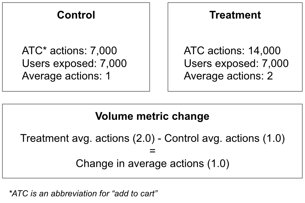
In the example above, assuming the volume change proves to be statistically significant, the treatment group can be said to have increased the average number of ATC actions by 100%. Another way to say this is that users in the treatment group on average make the ATC action one more time than those in control. Calculating a metric change using volume can create a powerful statement, although there is a higher likelihood of bias when using it. Since we are using an average we could be disproportionately weighing a single users influence or even worse a spammer / bot. This can be mitigated with techniques like winsorization but there is still room for bias.

Propensity analysis

The likelihood a user completed a specific action would be known as the user’s propensity for said action. The mathematical representation would be the number of unique user actions divided by the number of users. This metric will never exceed 100%. Let’s take a look at an example using the same data as before.

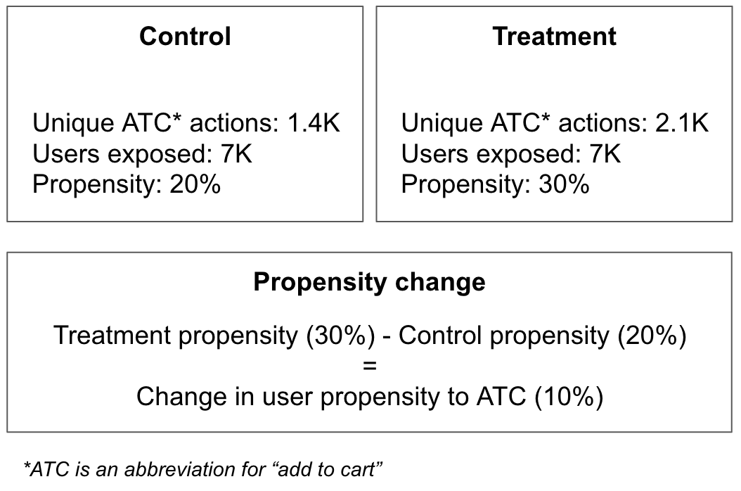
In the example above, assuming the propensity change proves to be statistically significant, the treatment group can be said to have increased the likelihood for a user to ATC by 50%. Another way to say this is that an additional 1 out of 10 users will add to cart within the treatment group when compared with control. Calculating a metric change using propensity has some advantages for a growth team. When looking at propensity it weighs marginal, new and core users equally. Often we see core and power users performing the most actions in an experiment. Since these super users already comprehend the value of the product and are using it efficiently should we be double counting them like in a volume analysis? For example if super users took 10x more actions than other users in an experiment to boost comprehension does a volume analysis make sense? In this case certainly not. With this point said judgement is certainly required when choosing which measurement analysis to focus on.

Measuring affected population

Since experimentation is usually the primary tool for measuring metric changes most folks will also use the number of users who joined during the experiment to calculate the total affected population. This is the right idea, but doing it improperly can lead to biased decision making. Specifically, taking the population too early in the formation of the experiment join curve can seriously understate the impact of a feature change.

Experiment join curve

When a user is exposed to an experiment for the first time it can be said they have “joined” the experiment. As more users join the cumulative amount can be plotted over time creating an experiment join curve.

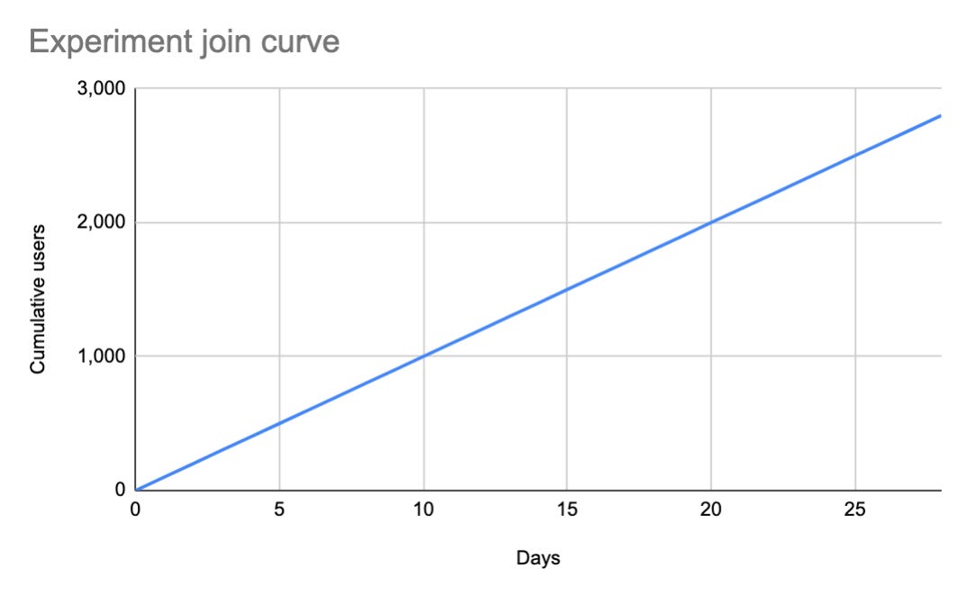
The above curve is linear and shows users join at a constant rate, but this isn’t always the case.

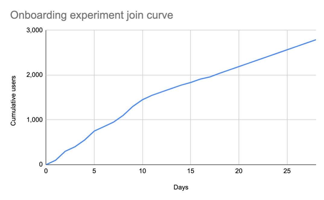
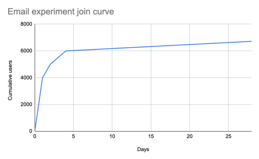
In these two different curves we can see that depending on the experiment the join curve can be wildly different. In the example of an email experiment we see that most of the users join the experiment immediately, while in the onboarding experiment it takes weeks to gain critical mass. So will an email experiment always have much higher impact since the population is greater? If we constrain our view to a short period of time, it will be difficult to justify focusing on onboarding experiments which will have a lower potential for impact. But what happens if we wait longer and see how the experiment join curve ends up over time?

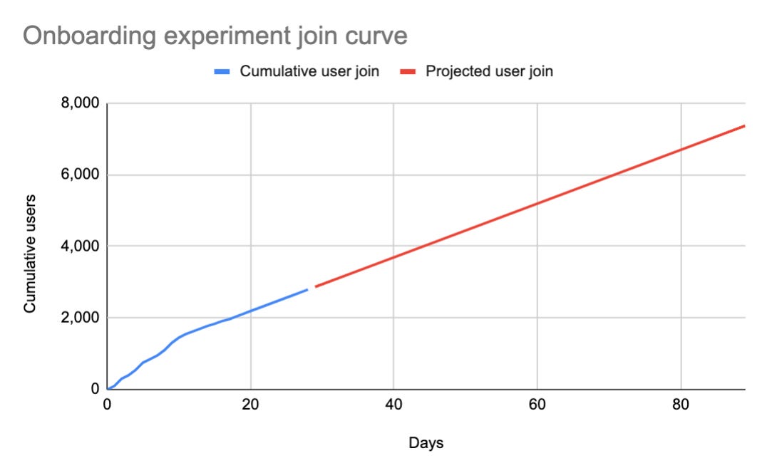
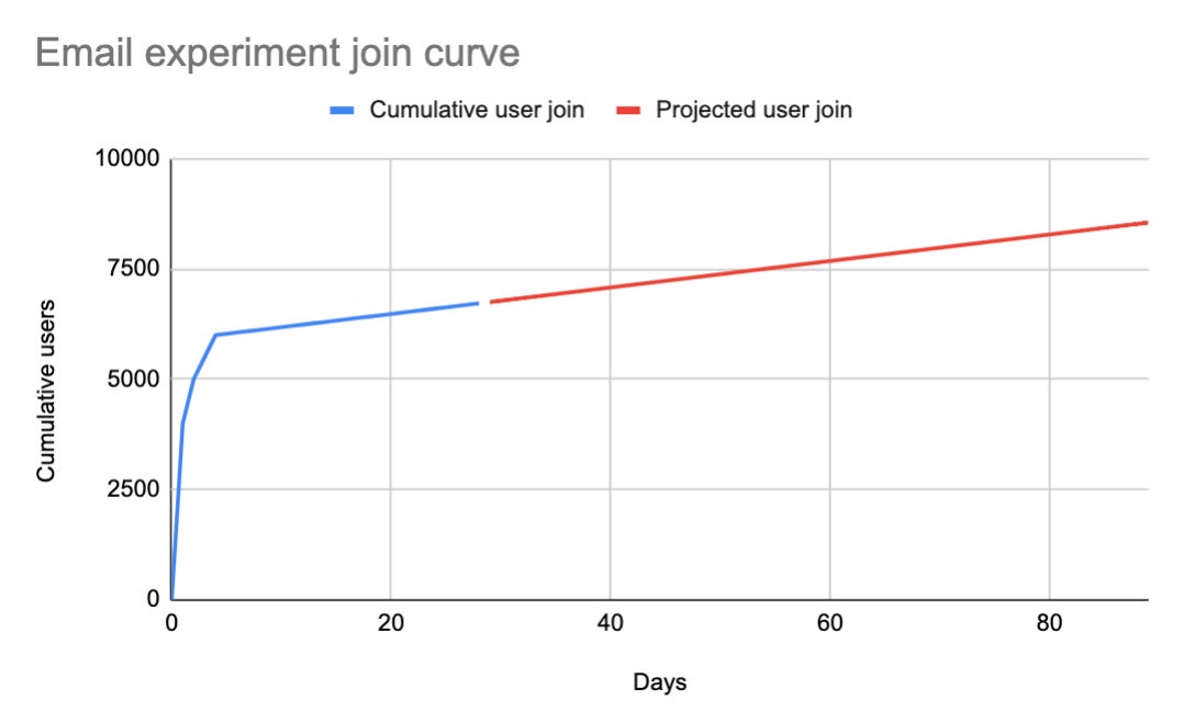
One way to see a longer time frame is to wait and actually get results. Often waiting an additional two months for measurement purposes is untenable. So instead a product team can decide to forecast the next 2 months of data by simply following the shape of the curve. In the examples above we did just that.

The email experiment projected population will increase by about 30% but the onboarding experiment now has almost 3x the population leading to a massive increase in the impact. For a mature product it is essential to look at populations over a longer period of time when judging impact, otherwise the product impact methodology will bias towards experiments with larger existing populations of users.

As can be seen in the projected curves above, this is a way to mitigate the potential for population bias. On the other hand this presents modeling risk, since this is just a prediction of future populations. In my view this tradeoff is worth it, assuming the modeler stays conservative and prudent in it’s design. The risk can be further mitigated by dedicating more resources to building better and more accurate models.

Final thoughts

While the benefits of quantifying product impact have been explained, I need to caution how it can be misinterpreted. Being metrics driven is a fantastic skill in any toolkit but it is not an excuse to abandon the user’s experience. It can be tempting to narrow mindedly chase after metric impact but this can ultimately lead to user backlash if a product team isn’t careful. Taking a balanced approach that weighs the considerations of each is why product owners and design leads are so valuable. The best products are created when a team balances insights from data along with qualitative feedback from a user’s experience.

Thanks for reading this post and special thanks to Meeka and Pam for reviewing and giving valuable feedback. If you are interested in more content like this please subscribe!